
rao1999: Predictive coding in the visual cortex: a functional interpretation of some extra-classical receptive-field effects
\( \newcommand{\states}{\mathcal{S}} \newcommand{\actions}{\mathcal{A}} \newcommand{\observations}{\mathcal{O}} \newcommand{\rewards}{\mathcal{R}} \newcommand{\traces}{\mathbf{e}} \newcommand{\transition}{P} \newcommand{\reals}{\mathbb{R}} \newcommand{\naturals}{\mathbb{N}} \newcommand{\complexs}{\mathbb{C}} \newcommand{\field}{\mathbb{F}} \newcommand{\numfield}{\mathbb{F}} \newcommand{\expected}{\mathbb{E}} \newcommand{\var}{\mathbb{V}} \newcommand{\by}{\times} \newcommand{\partialderiv}[2]{\frac{\partial #1}{\partial #2}} \newcommand{\defineq}{\stackrel{{\tiny\mbox{def}}}{=}} \newcommand{\defeq}{\stackrel{{\tiny\mbox{def}}}{=}} \newcommand{\eye}{\Imat} \newcommand{\hadamard}{\odot} \newcommand{\trans}{\top} \newcommand{\inv}{{-1}} \newcommand{\argmax}{\operatorname{argmax}} \newcommand{\Prob}{\mathbb{P}} \newcommand{\avec}{\mathbf{a}} \newcommand{\bvec}{\mathbf{b}} \newcommand{\cvec}{\mathbf{c}} \newcommand{\dvec}{\mathbf{d}} \newcommand{\evec}{\mathbf{e}} \newcommand{\fvec}{\mathbf{f}} \newcommand{\gvec}{\mathbf{g}} \newcommand{\hvec}{\mathbf{h}} \newcommand{\ivec}{\mathbf{i}} \newcommand{\jvec}{\mathbf{j}} \newcommand{\kvec}{\mathbf{k}} \newcommand{\lvec}{\mathbf{l}} \newcommand{\mvec}{\mathbf{m}} \newcommand{\nvec}{\mathbf{n}} \newcommand{\ovec}{\mathbf{o}} \newcommand{\pvec}{\mathbf{p}} \newcommand{\qvec}{\mathbf{q}} \newcommand{\rvec}{\mathbf{r}} \newcommand{\svec}{\mathbf{s}} \newcommand{\tvec}{\mathbf{t}} \newcommand{\uvec}{\mathbf{u}} \newcommand{\vvec}{\mathbf{v}} \newcommand{\wvec}{\mathbf{w}} \newcommand{\xvec}{\mathbf{x}} \newcommand{\yvec}{\mathbf{y}} \newcommand{\zvec}{\mathbf{z}} \newcommand{\Amat}{\mathbf{A}} \newcommand{\Bmat}{\mathbf{B}} \newcommand{\Cmat}{\mathbf{C}} \newcommand{\Dmat}{\mathbf{D}} \newcommand{\Emat}{\mathbf{E}} \newcommand{\Fmat}{\mathbf{F}} \newcommand{\Gmat}{\mathbf{G}} \newcommand{\Hmat}{\mathbf{H}} \newcommand{\Imat}{\mathbf{I}} \newcommand{\Jmat}{\mathbf{J}} \newcommand{\Kmat}{\mathbf{K}} \newcommand{\Lmat}{\mathbf{L}} \newcommand{\Mmat}{\mathbf{M}} \newcommand{\Nmat}{\mathbf{N}} \newcommand{\Omat}{\mathbf{O}} \newcommand{\Pmat}{\mathbf{P}} \newcommand{\Qmat}{\mathbf{Q}} \newcommand{\Rmat}{\mathbf{R}} \newcommand{\Smat}{\mathbf{S}} \newcommand{\Tmat}{\mathbf{T}} \newcommand{\Umat}{\mathbf{U}} \newcommand{\Vmat}{\mathbf{V}} \newcommand{\Wmat}{\mathbf{W}} \newcommand{\Xmat}{\mathbf{X}} \newcommand{\Ymat}{\mathbf{Y}} \newcommand{\Zmat}{\mathbf{Z}} \newcommand{\Sigmamat}{\boldsymbol{\Sigma}} \newcommand{\identity}{\Imat} \newcommand{\thetavec}{\boldsymbol{\theta}} \newcommand{\phivec}{\boldsymbol{\phi}} \newcommand{\muvec}{\boldsymbol{\mu}} \newcommand{\sigmavec}{\boldsymbol{\sigma}} \newcommand{\jacobian}{\mathbf{J}} \newcommand{\ind}{\perp!!!!\perp} \newcommand{\bigoh}{\text{O}} \)
- tags
- Predictive Processing, Brain
- source
- paper
- authors
- Rao, R. P. N., & Ballard, D. H.
- year
- 1999
This paper introduces predictive coding in which feedback connections from a higher- to a lower-order visual cortical area carry predictions of lower-level neural activities. The feedforward connections carry residual errors between the predictions and the actual lower-level activities.
First, there is a curious property of neurons which respond optimally to line segments of a particular length (reported in prior studies). These neurons have the property of endstopping (or end-inhibition): a vigorous response to an optimally oriented line segment is reduced or eliminated when the same stimulus extends beyond the neuron’s classical receptive field (RF). There have been several proposed explanations for this behaviour, but in this paper they present simulations which suggest the extra-classical RF effects may result directly from predictive coding of natural images.
Results
Hierarchical Predictive Coding Model
Each level in the hierarchical model network attempts to predict the responses at the next lower level via feedback connections. The error between the prediction and the actual response is then sent back to the higher level via feedforward connections.
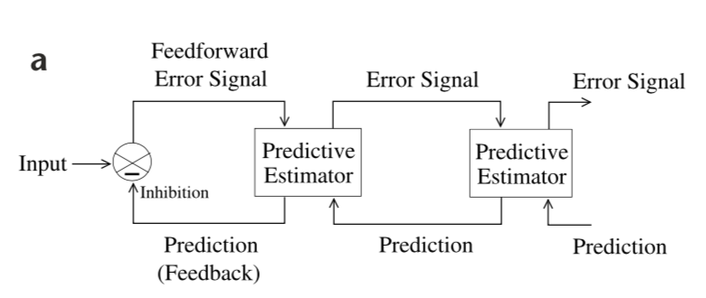
Figure 1: General Architecture of the hierarchical predictive coding model.
The prediction and error mechanisms occur concurrently throughout the hierarchy (top-down information influences bottom-up). Lower levels operate on smaller spatial (and possibly temporal scales) regions of th image, and the effective RF size of units increases progressively until the highest level’s RF spans the totality of the image. Like all models, the underlying assumption is that the external environment generates natural signals hierarchically via interacting hidden physical causes (partial observability). The goal of the visual system is to optimally estimate the hidden variable at each scale of the input image.
Hierarchical Predictive Coding of Natural Images
The model described in the above section suggests feedback connections from a higher area to a lower area carry prediction of expected neural activity, whereas feedforward connections convey the residual activity (or unexplained activations) not predicted by the higher area. This was tested through simulation using a three-level hierarchical network of predictive estimators. The details on how this model is constructed and trained are left to the methods section sec:rao1999:methods, but here we give a high level overview:
- The hierarchical internal model is trained by maximizing the posterior probability of generating the observed natural images.
- The internal model is encoded in a distributed manner within the synapses of model neurons at each level
- The weights of a neuron encode a single basis vector that, in conjunction with other basis vectors, predicts lower-level inputs. Example: The image input at the zeroth level can be predicted as an appropriate linear combination of the first-level basis vectors. The weighting coefficient for the kth basis vector is given by the response of the kth neuron in the first level.
- These are simulated by a first-order differential equation implementing the prediction and error-correction cycle.
- For any given input, the network converges to a set of neuronal responses optimal for predicting the input, which are used to adapt the synaptic basis vectors.
The resulting weights resembled the Gabor or difference-of-Gaussians filters (studied prior) when using a Gaussian weighting profile to model the input. When using a sparse prior distribution the wavelet-like basis vectors code for local oriented structures rather than being centered in the input window.
Endstopped Responses Interpreted as Error Signals
They show that they are able to illicit large error responses (feedback responses) based on the lack of contextual information (i.e. a bar within a single neurons RF or across multiple RFs). With contextual information the response of specific neurons are inhibited due to the input being predicted at higher-levels (i.e. the error-signal of the feed-forward connections are small). This is similar to the endstopped property of neurons discussed earlier.
Predictive Feedback and Extra-Classical RF Effects
They computed the percentage of endstopping (really the inverse as they report \(\%\) maximum response). They find that feedback connections are critical to the endstopping phenomenon in their model.
Other Extra-Classical RF Effects in the Model
Discussion
- The simulations suggest certain extra-classical RF effects could be an emergent property of the cortex using an efficient hierarchical and predictive strategy for encoding natural images.
- These simulations also show that extra-classical RF effects can occur under predictive coding with either Gaussian or sparse kurtotic prior distributions for the network activities.
- These general ideas may help explain certain responses in other brain regions. Examples:
- Some neurons in MT are suppressed when the direction of stimulus motion in the surrounding region matches that in the center of the classical RF.
- Certain neurons in the anterior inferotemporal (IT) cortex of alert behaving monkeys fire vigorously whenever a presented test stimulus does not match the item held in memory (showing little activation in the case of a match)
- The generation and subtraction of sensory expectations from actual inputs in cerebellum-like structures.
- The responses of dopaminergic neurons projecting to the cortex and striatum from the midbrain can often be characterized as encoding reward prediction errors: large responses are elicited whenever actual rewards do not match the predicted reward in behavioral tasks
Methods
They characterize each image \(\Imat\) (or higher level inputs) to have a relationship
\[\Imat = f(\Umat \rvec) + \nvec\]
- \(\Imat\) is the image (or a part of an image)
- \(f\) is some activation function
- \(\Umat\) is a matrix with each column representing a basis vector for generating images
- \(\rvec\) are the causes of the image
- \(\nvec\) some stochastic noise process.
We assume the causes \(\rvec\) can be represented by a set of higher-level causes \(\rvec^h\) potentially representing higher level abstractions.
\[\rvec = \rvec^{td} + \nvec^{td}\]
where
\[\rvec^{td} = f(\Umat^h \rvec^h)\].
We must limit the size of the image (or the main predictive signal) for a single predictive coding cell, and only consider a local region when developing predictions. Higher level cells will represent more abstract concepts and thus will span a larger image width. To allow prediction in time, the model can be exteded using a set of recurrent synaptic weights.
Optimization function
The goal is to estimate the coefficients \(\rvec\) for a given image and learn appropriate basis vectors \(\Umat_j\) for each hierarchical level. Assuming the noise terms \(\nvec\) and \(\nvec^{td}\) are zero mean Gaussians, we can write the optimization function:
\[E_1 = \frac{1}{\sigmavec^2} (\Imat - f(\Umat \rvec))^\trans (\Imat - f(\Umat \rvec)) + \frac{1}{\sigmavec_{td}^2} (\rvec - \rvec^td)^\trans (\rvec - \rvec^td)\]
For their simulations they also use prior distributions over the causes and synaptic weights making the final error
\[E = E_1 + g(\rvec) + h(\Umat)\].
Where g and h are the negative logarithms of the prior probabilities of \(\rvec\) and \(\Umat\) respectively (in their simulations they use Gaussian prior distributions \(g(\rvec) = \alpha \sum_i \rvec_i^2\)). Through bayes therom it can also be seen that minimizing \(E\) is equivalent to maximizing the posterior probability of the model parameters given the input data. For details on how to optimize this function through gradient descent see the paper.