
weng2021how: How to Train Really Large Models on Many GPUs? | Lil'Log
\( \newcommand{\states}{\mathcal{S}} \newcommand{\actions}{\mathcal{A}} \newcommand{\observations}{\mathcal{O}} \newcommand{\rewards}{\mathcal{R}} \newcommand{\traces}{\mathbf{e}} \newcommand{\transition}{P} \newcommand{\reals}{\mathbb{R}} \newcommand{\naturals}{\mathbb{N}} \newcommand{\complexs}{\mathbb{C}} \newcommand{\field}{\mathbb{F}} \newcommand{\numfield}{\mathbb{F}} \newcommand{\expected}{\mathbb{E}} \newcommand{\var}{\mathbb{V}} \newcommand{\by}{\times} \newcommand{\partialderiv}[2]{\frac{\partial #1}{\partial #2}} \newcommand{\defineq}{\stackrel{{\tiny\mbox{def}}}{=}} \newcommand{\defeq}{\stackrel{{\tiny\mbox{def}}}{=}} \newcommand{\eye}{\Imat} \newcommand{\hadamard}{\odot} \newcommand{\trans}{\top} \newcommand{\inv}{{-1}} \newcommand{\argmax}{\operatorname{argmax}} \newcommand{\Prob}{\mathbb{P}} \newcommand{\avec}{\mathbf{a}} \newcommand{\bvec}{\mathbf{b}} \newcommand{\cvec}{\mathbf{c}} \newcommand{\dvec}{\mathbf{d}} \newcommand{\evec}{\mathbf{e}} \newcommand{\fvec}{\mathbf{f}} \newcommand{\gvec}{\mathbf{g}} \newcommand{\hvec}{\mathbf{h}} \newcommand{\ivec}{\mathbf{i}} \newcommand{\jvec}{\mathbf{j}} \newcommand{\kvec}{\mathbf{k}} \newcommand{\lvec}{\mathbf{l}} \newcommand{\mvec}{\mathbf{m}} \newcommand{\nvec}{\mathbf{n}} \newcommand{\ovec}{\mathbf{o}} \newcommand{\pvec}{\mathbf{p}} \newcommand{\qvec}{\mathbf{q}} \newcommand{\rvec}{\mathbf{r}} \newcommand{\svec}{\mathbf{s}} \newcommand{\tvec}{\mathbf{t}} \newcommand{\uvec}{\mathbf{u}} \newcommand{\vvec}{\mathbf{v}} \newcommand{\wvec}{\mathbf{w}} \newcommand{\xvec}{\mathbf{x}} \newcommand{\yvec}{\mathbf{y}} \newcommand{\zvec}{\mathbf{z}} \newcommand{\Amat}{\mathbf{A}} \newcommand{\Bmat}{\mathbf{B}} \newcommand{\Cmat}{\mathbf{C}} \newcommand{\Dmat}{\mathbf{D}} \newcommand{\Emat}{\mathbf{E}} \newcommand{\Fmat}{\mathbf{F}} \newcommand{\Gmat}{\mathbf{G}} \newcommand{\Hmat}{\mathbf{H}} \newcommand{\Imat}{\mathbf{I}} \newcommand{\Jmat}{\mathbf{J}} \newcommand{\Kmat}{\mathbf{K}} \newcommand{\Lmat}{\mathbf{L}} \newcommand{\Mmat}{\mathbf{M}} \newcommand{\Nmat}{\mathbf{N}} \newcommand{\Omat}{\mathbf{O}} \newcommand{\Pmat}{\mathbf{P}} \newcommand{\Qmat}{\mathbf{Q}} \newcommand{\Rmat}{\mathbf{R}} \newcommand{\Smat}{\mathbf{S}} \newcommand{\Tmat}{\mathbf{T}} \newcommand{\Umat}{\mathbf{U}} \newcommand{\Vmat}{\mathbf{V}} \newcommand{\Wmat}{\mathbf{W}} \newcommand{\Xmat}{\mathbf{X}} \newcommand{\Ymat}{\mathbf{Y}} \newcommand{\Zmat}{\mathbf{Z}} \newcommand{\Sigmamat}{\boldsymbol{\Sigma}} \newcommand{\identity}{\Imat} \newcommand{\epsilonvec}{\boldsymbol{\epsilon}} \newcommand{\thetavec}{\boldsymbol{\theta}} \newcommand{\phivec}{\boldsymbol{\phi}} \newcommand{\muvec}{\boldsymbol{\mu}} \newcommand{\sigmavec}{\boldsymbol{\sigma}} \newcommand{\jacobian}{\mathbf{J}} \newcommand{\ind}{\perp!!!!\perp} \newcommand{\bigoh}{\text{O}} \)
- tags
- Machine Learning
- source
- https://lilianweng.github.io/posts/2021-09-25-train-large/
- authors
- Weng, L.
- year
- 2021
I am reading this to learn a little bit about the computational model for training large models. This is primarily for the modl interview, but of interest generally.
Data Parallelism
If the model size is too large (i.e. larger than the size of a single GPU node’s memory) naive DP won’t work (i.e. copy the same models across multiple GPU nodes. One can offload temporarily unused parameters to the CPU to work with the limited GPU memory using methods like GeePS (Cui et al. 2016).
At the end of each minibatch the workers need to synchronize gradients/weights to avoid staleness.
- Bulk synchronous parallels (BSP): Workers sync data at the end of every minibatch. Prevents weight staleness, but can cause waiting between nodes.
- Asynchronous parallel (ASP): Every GPU worker processes the data asynchronously. This can lead to stale weights lowering the statistical learning efficiency. May not speed up training time.
There is a middle ground where gradients are globally once every x iterations (where \(x>1\). This is called “gradient accumulation” in Distribution Data Parallel in PyTorch.
Model Parallelism
A naive implementation allocates one layer per worker. This generates an obvious “bib bubble of waiting time” which severely under-utilizes computation. This can be seen in the figure <mp_naive>.
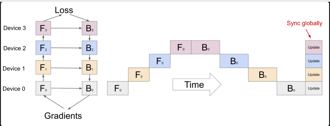
Figure 1: A naive model parallelism setup where the model is vertically split into 4 partitions (i.e. each layer is in a seperate worker).
Pipeline Parallelism
We can use Pipeline Parallelism to combine both model parallelism with data parallelism. The core idea is broken into a few pieces:
- Split one minibatch into multiple microbatches and enable each stage worker to process one microbatch simultaneously.
- Inter-workder communication only transfers activations (forward) and gradients (backward). The specific scheduling is different per different approaches (see below).
pipeline depth: this is the number of workers used.
Some notable algorithms:
- GPipe (Huang et al. 2019): gradients of the microbatches are aggregated and applied synchronously at the end.
- PipeDream (Narayanan et al. 2019): Schedules each worker to alternatively process the forward and backward pass. This means the method doesn’t have an end of batch gradient synchronization, which could lower the learning efficiency. This can be dealt with in a few ways like weight stashing or vertical sync.
- PipeDream-flush: adds globally synchronized pipeline flush.
- PipeDream-2BW (Narayanan et al. 2021): Maintains only two versions of model weights. This generates a new model version every k microbatches and k should be larger then the pipeline depth.
Tensor Parallelism
This parallelizes horizontally where layers can be computed on several nodes. This can be combined with pipeline and data parallelism.
Mixture-of-Experts
A mixture of weak models results in a strong model (Shazeer et al. 2017).