
Power Systems Control
\( \newcommand{\states}{\mathcal{S}} \newcommand{\actions}{\mathcal{A}} \newcommand{\observations}{\mathcal{O}} \newcommand{\rewards}{\mathcal{R}} \newcommand{\traces}{\mathbf{e}} \newcommand{\transition}{P} \newcommand{\reals}{\mathbb{R}} \newcommand{\naturals}{\mathbb{N}} \newcommand{\complexs}{\mathbb{C}} \newcommand{\field}{\mathbb{F}} \newcommand{\numfield}{\mathbb{F}} \newcommand{\expected}{\mathbb{E}} \newcommand{\var}{\mathbb{V}} \newcommand{\by}{\times} \newcommand{\partialderiv}[2]{\frac{\partial #1}{\partial #2}} \newcommand{\defineq}{\stackrel{{\tiny\mbox{def}}}{=}} \newcommand{\defeq}{\stackrel{{\tiny\mbox{def}}}{=}} \newcommand{\eye}{\Imat} \newcommand{\hadamard}{\odot} \newcommand{\trans}{\top} \newcommand{\inv}{{-1}} \newcommand{\argmax}{\operatorname{argmax}} \newcommand{\Prob}{\mathbb{P}} \newcommand{\avec}{\mathbf{a}} \newcommand{\bvec}{\mathbf{b}} \newcommand{\cvec}{\mathbf{c}} \newcommand{\dvec}{\mathbf{d}} \newcommand{\evec}{\mathbf{e}} \newcommand{\fvec}{\mathbf{f}} \newcommand{\gvec}{\mathbf{g}} \newcommand{\hvec}{\mathbf{h}} \newcommand{\ivec}{\mathbf{i}} \newcommand{\jvec}{\mathbf{j}} \newcommand{\kvec}{\mathbf{k}} \newcommand{\lvec}{\mathbf{l}} \newcommand{\mvec}{\mathbf{m}} \newcommand{\nvec}{\mathbf{n}} \newcommand{\ovec}{\mathbf{o}} \newcommand{\pvec}{\mathbf{p}} \newcommand{\qvec}{\mathbf{q}} \newcommand{\rvec}{\mathbf{r}} \newcommand{\svec}{\mathbf{s}} \newcommand{\tvec}{\mathbf{t}} \newcommand{\uvec}{\mathbf{u}} \newcommand{\vvec}{\mathbf{v}} \newcommand{\wvec}{\mathbf{w}} \newcommand{\xvec}{\mathbf{x}} \newcommand{\yvec}{\mathbf{y}} \newcommand{\zvec}{\mathbf{z}} \newcommand{\Amat}{\mathbf{A}} \newcommand{\Bmat}{\mathbf{B}} \newcommand{\Cmat}{\mathbf{C}} \newcommand{\Dmat}{\mathbf{D}} \newcommand{\Emat}{\mathbf{E}} \newcommand{\Fmat}{\mathbf{F}} \newcommand{\Gmat}{\mathbf{G}} \newcommand{\Hmat}{\mathbf{H}} \newcommand{\Imat}{\mathbf{I}} \newcommand{\Jmat}{\mathbf{J}} \newcommand{\Kmat}{\mathbf{K}} \newcommand{\Lmat}{\mathbf{L}} \newcommand{\Mmat}{\mathbf{M}} \newcommand{\Nmat}{\mathbf{N}} \newcommand{\Omat}{\mathbf{O}} \newcommand{\Pmat}{\mathbf{P}} \newcommand{\Qmat}{\mathbf{Q}} \newcommand{\Rmat}{\mathbf{R}} \newcommand{\Smat}{\mathbf{S}} \newcommand{\Tmat}{\mathbf{T}} \newcommand{\Umat}{\mathbf{U}} \newcommand{\Vmat}{\mathbf{V}} \newcommand{\Wmat}{\mathbf{W}} \newcommand{\Xmat}{\mathbf{X}} \newcommand{\Ymat}{\mathbf{Y}} \newcommand{\Zmat}{\mathbf{Z}} \newcommand{\Sigmamat}{\boldsymbol{\Sigma}} \newcommand{\identity}{\Imat} \newcommand{\epsilonvec}{\boldsymbol{\epsilon}} \newcommand{\thetavec}{\boldsymbol{\theta}} \newcommand{\phivec}{\boldsymbol{\phi}} \newcommand{\muvec}{\boldsymbol{\mu}} \newcommand{\sigmavec}{\boldsymbol{\sigma}} \newcommand{\jacobian}{\mathbf{J}} \newcommand{\ind}{\perp!!!!\perp} \newcommand{\bigoh}{\text{O}} \)
Projects
Questions
Notes/Literature
Common terms
- Distributed Generation Units
- Energy Storage Systems
- Point of Common Coupling
- Voltage Source Converters
- Swing Equation
-
Phasor Measurement Units
- TODO Overview of history of PMUs (Phadke 2002)
- TODO Government installing PMUs (“New Technology Can Improve Electric Power System Efficiency and Reliability - U.S. Energy Information Administration (EIA)” 2025).
Microgrid Control
A microgrid can be though of a cluster of loads, Distributed Generation Units and Energy Storage Systems operated in coordination to reliably supply electricty, connected to the host power system at the distribution level at a single point of connection, i.e. the Point of Common Coupling.
- TODO (Olivares et al. 2014)
-
Some links
- An example model of a small scale microgrid: link
TODO (Dommel 1969)
Problem Settings/Use Cases
-
Electro-Magnetic Transient Simulation
Electro Magnetic Transient Simulation
- TODO (Zhang et al. 1997)
- Power Flow
- Optimal Power Flow
-
Stability Analysis
Along with transient stability assessment..
-
Co-Simulation
Joint simulation of loosely coupled stand-alone sub-simulators
Examples/Benchmarks
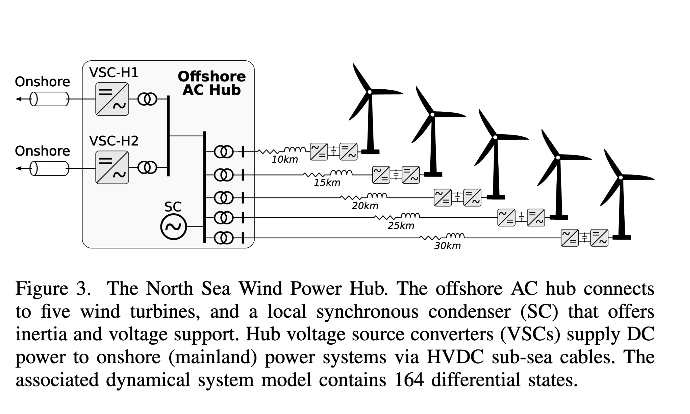
The North Sea Wind Power Hub
Depicted below, this model represents a realistic example of an emerging converter-dominated system that must integrate securely into the legacy bulk power grid. The objective is to optimally tune the control parameters and determine the power dispatch of the NSWPH system under small-signal stability and N-1 security constraints.
The below figure depicts:
- 5 wind farms,
- a synchronous condenser,
- and two HVDC Voltage Source Converters
When planning dispatch of the system, operators are assumed to have control over the active and reactive power set points of the turbines. In the future, operators may also depend on the wind hubs to provide both primary frequency and primary voltage control support services. We assume operators have the capacity to adjust the droop parameters which determine the system’s participation in both primary frequency and primary voltage control.
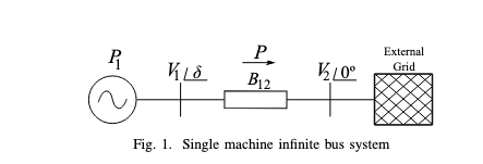
Single Machine Infinite Bus system
This is an extremely simple power bus with a single generator and infinite external grid which has a constant draw of power without a shift in voltage or angle (very idealized system).
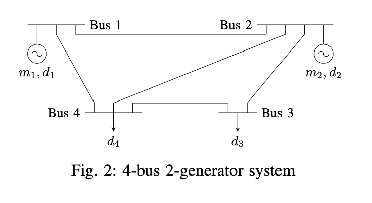
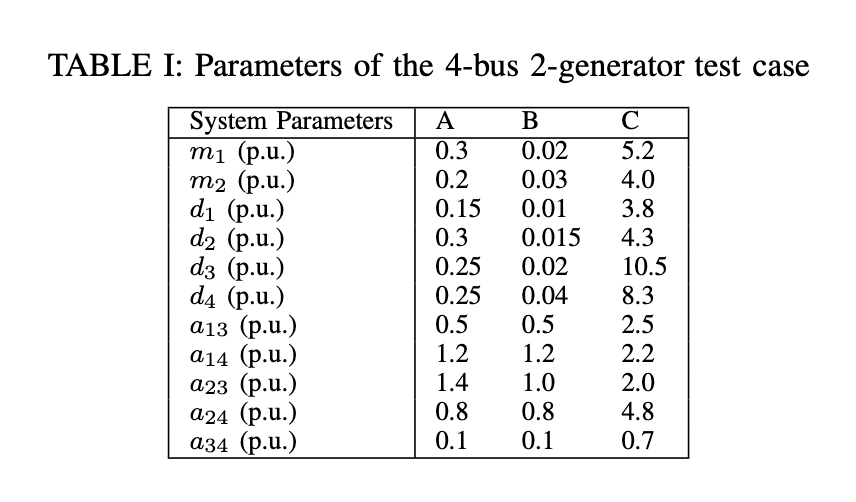
4-Bus 2-Generator System
Described in (Stiasny, Misyris, and Chatzivasileiadis 2021). With governing dynamics \[ m_k \ddot{\delta}_k + d_k \dot{\delta}_k + \sum_j B_{kj} V_k V_j \text{sin}(\delta_k - \delta_j) - P_k = 0 \]
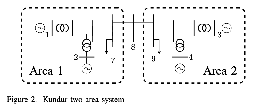
Kundur Two-area system
First came across in (Stiasny, Misyris, and Chatzivasileiadis 2023). Originally described in https://www.taylorfrancis.com/chapters/edit/10.4324/b12113-10/power-system-stability-prabha-kundur.
Governing equations:
\begin{align} \dot{\delta}_i &= \omega_i - \omega_0 \\ \dot{\omega}_i &= \frac{\omega_0}{2H_i} \left ( P_i^{\text{set}} + \Delta P_i - \sum_j \frac{V_i V_j}{X_{ij}} \sin(\delta_i - \delta_j) \right ) \\ \dot{\delta}_i &= \frac{1}{D_i} \left ( P_i^{\text{set}} + \Delta P_i - \sum_j \frac{V_i V_j}{X_{ij}} \sin(\delta_i - \delta_j) \right ) \end{align}
IEEE Bus Systems
- IEEE 14 Bus System
- IEEE 33 Bus System
- IEEE 118 Bus System
PanTaGruEl
A simulation of the European power grid