
guo2016convolutional: Convolutional Neural Networks for Steady Flow Approximation
\( \newcommand{\states}{\mathcal{S}} \newcommand{\actions}{\mathcal{A}} \newcommand{\observations}{\mathcal{O}} \newcommand{\rewards}{\mathcal{R}} \newcommand{\traces}{\mathbf{e}} \newcommand{\transition}{P} \newcommand{\reals}{\mathbb{R}} \newcommand{\naturals}{\mathbb{N}} \newcommand{\complexs}{\mathbb{C}} \newcommand{\field}{\mathbb{F}} \newcommand{\numfield}{\mathbb{F}} \newcommand{\expected}{\mathbb{E}} \newcommand{\var}{\mathbb{V}} \newcommand{\by}{\times} \newcommand{\partialderiv}[2]{\frac{\partial #1}{\partial #2}} \newcommand{\defineq}{\stackrel{{\tiny\mbox{def}}}{=}} \newcommand{\defeq}{\stackrel{{\tiny\mbox{def}}}{=}} \newcommand{\eye}{\Imat} \newcommand{\hadamard}{\odot} \newcommand{\trans}{\top} \newcommand{\inv}{{-1}} \newcommand{\argmax}{\operatorname{argmax}} \newcommand{\Prob}{\mathbb{P}} \newcommand{\avec}{\mathbf{a}} \newcommand{\bvec}{\mathbf{b}} \newcommand{\cvec}{\mathbf{c}} \newcommand{\dvec}{\mathbf{d}} \newcommand{\evec}{\mathbf{e}} \newcommand{\fvec}{\mathbf{f}} \newcommand{\gvec}{\mathbf{g}} \newcommand{\hvec}{\mathbf{h}} \newcommand{\ivec}{\mathbf{i}} \newcommand{\jvec}{\mathbf{j}} \newcommand{\kvec}{\mathbf{k}} \newcommand{\lvec}{\mathbf{l}} \newcommand{\mvec}{\mathbf{m}} \newcommand{\nvec}{\mathbf{n}} \newcommand{\ovec}{\mathbf{o}} \newcommand{\pvec}{\mathbf{p}} \newcommand{\qvec}{\mathbf{q}} \newcommand{\rvec}{\mathbf{r}} \newcommand{\svec}{\mathbf{s}} \newcommand{\tvec}{\mathbf{t}} \newcommand{\uvec}{\mathbf{u}} \newcommand{\vvec}{\mathbf{v}} \newcommand{\wvec}{\mathbf{w}} \newcommand{\xvec}{\mathbf{x}} \newcommand{\yvec}{\mathbf{y}} \newcommand{\zvec}{\mathbf{z}} \newcommand{\Amat}{\mathbf{A}} \newcommand{\Bmat}{\mathbf{B}} \newcommand{\Cmat}{\mathbf{C}} \newcommand{\Dmat}{\mathbf{D}} \newcommand{\Emat}{\mathbf{E}} \newcommand{\Fmat}{\mathbf{F}} \newcommand{\Gmat}{\mathbf{G}} \newcommand{\Hmat}{\mathbf{H}} \newcommand{\Imat}{\mathbf{I}} \newcommand{\Jmat}{\mathbf{J}} \newcommand{\Kmat}{\mathbf{K}} \newcommand{\Lmat}{\mathbf{L}} \newcommand{\Mmat}{\mathbf{M}} \newcommand{\Nmat}{\mathbf{N}} \newcommand{\Omat}{\mathbf{O}} \newcommand{\Pmat}{\mathbf{P}} \newcommand{\Qmat}{\mathbf{Q}} \newcommand{\Rmat}{\mathbf{R}} \newcommand{\Smat}{\mathbf{S}} \newcommand{\Tmat}{\mathbf{T}} \newcommand{\Umat}{\mathbf{U}} \newcommand{\Vmat}{\mathbf{V}} \newcommand{\Wmat}{\mathbf{W}} \newcommand{\Xmat}{\mathbf{X}} \newcommand{\Ymat}{\mathbf{Y}} \newcommand{\Zmat}{\mathbf{Z}} \newcommand{\Sigmamat}{\boldsymbol{\Sigma}} \newcommand{\identity}{\Imat} \newcommand{\epsilonvec}{\boldsymbol{\epsilon}} \newcommand{\thetavec}{\boldsymbol{\theta}} \newcommand{\phivec}{\boldsymbol{\phi}} \newcommand{\muvec}{\boldsymbol{\mu}} \newcommand{\sigmavec}{\boldsymbol{\sigma}} \newcommand{\jacobian}{\mathbf{J}} \newcommand{\ind}{\perp!!!!\perp} \newcommand{\bigoh}{\text{O}} \)
- tags
- Data Driven PDE Solvers, Neural Network, Machine Learning, Supervised Learning
- source
- https://dl.acm.org/doi/10.1145/2939672.2939738
- authors
- Guo, X., Li, W., & Iorio, F.
- year
- 2016
This paper proposes a Convolutional Neural Network approach for approximating the laminar flow of a fluid around a geometry.
Input: The paper defines its input space based on the distance of a point (discretized from the real space) to a defined geometry with a sign determining if it is inside or outside the boundary (negative if inside, positive if outside, and zero if on the boundary). see the following example:
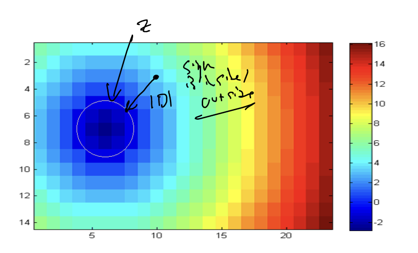
Figure 1: A discrete Signed Distance Function representation of a circle shape in a 23x14 Cartesian grid. Notation by me.
In the above your can see how the geometry is defined by the white boundary, and the SDF is calculated based on the perpendicular distance to this point.
Architecture:
The input is then passed through a number of convolutional encoders, and then decoded into a CFD velocity field component (i.e. different outputs for each spacial component). The full details can be seen in the paper.
Data
The data is generated using Lattice Boltzmann Method using the geometry of the system. The output of the LCB simulation is used as the targets of the network w/ the SDF described above as the input.
Results
They show they can get significantly faster inference time for CFD with generic geometries as compared to LCB, with reasonable error.